CONCATENATE Excel Range (with and without separator)

In Excel, there are two ways to combine the contents of multiple cells:

• Excel CONCATENATE function (or the ampersand (&) operator)
• Excel TEXTJOIN function (new function in Excel if you have Office 365)

If you’re using Excel with Office 365 subscription, I suggest you click here to skip to the part where the TEXTJOIN function is covered.

If you’re not using Office 365, keep reading.

In its basic form, CONCATENATE function can join 2 or more characters of strings.

For example:

• =CONCATENATE(“Good”,”Morning”) will give you the result as GoodMorning
• =CONCATENATE(“Good”,” “, “Morning”) will give you the result as Good Morning
• =CONCATENATE(A1&A2) will give you the result as GoodMorning (where A1 has the text ‘Good’ in it and A2 has the text ‘Morning’.

While you can enter the reference one by one within the CONCATENATE function, it would not work if you enter the reference of multiple cells at once (as shown below):

For example, in the example above, while the formula used is =CONCATENATE(A1:A5), the result only shows ‘Today’ and doesn’t combine all the cells.

In this tutorial, I will show you how to combine multiple cells by using the CONCATENATE function.

Note: If you’re using Excel 2016, you can use the TEXTJOIN function that is built to combine multiple cells using a delimiter.

CONCATENATE Excel Range (Without any Separator)

Here are the steps to concatenate an Excel range without any separator (as shown in the pic):

1. Select the cell where you need the result.
2. Go to formula bar and enter =TRANSPOSE(A1:A5)
   • Based on your regional settings, you can also try =A1:A5 (instead of =TRANSPOSE(A1:A5))
3. Select the entire formula and press F9 (this converts the formula into values).
4. Remove the curly brackets from both ends.
5. Add =CONCATENATE( to the beginning of the text and end it with a round bracket).
6. Press Enter.

Doing this would combine the range of cells into one cell (as shown in the image above). Note that since we use any delimiter (such as comma or space), all the words are joined without any separator.

CONCATENATE Excel Ranges (With a Separator)

Here are the steps to concatenate an Excel Range with space as the separator (as shown in the pic):

1. Select the cell where you need the result.
2. Go to formula bar and enter =TRANSPOSE(A1:A5)&” “
   • Based on your regional settings, you can also try =A1:A5 (instead of =TRANSPOSE(A1:A5)).
3. Select the entire formula and press F9 (this converts the formula into values).
4. Remove the curly brackets from both ends.
5. Add =CONCATENATE( to the beginning of the text and end it with a round bracket).
6. Press Enter

Note that in this case, I used a space character as the separator (delimiter). If you want, you can use other separators such as a comma or hyphen.

CONCATENATE Excel Ranges (Using VBA)

Below is an example of the custom function I created using VBA (I named it CONCATENATEMULTIPLE) that will allow you to combine multiple cells as well as specify a separator/delimiter.

Here is the VBA code that will create this custom function to combine multiple cells:

Function CONCATENATEMULTIPLE(Ref As Range, Separator As String) As String
Dim Cell As Range
Dim Result As String
For Each Cell In Ref
 Result = Result & Cell.Value & Separator
Next Cell
CONCATENATEMULTIPLE = Left(Result, Len(Result) - 1)
End Function

Here are the steps to copy this code in Excel:

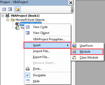
• Go to the Developer Tab and click on the Visual Basic icon (or use the keyboard shortcut Alt + F11).
• In the VB Editor, right-click on any of the objects and go to Insert and select Module.
• Copy paste the above code in the module code window.
• Close the VB Editor.

Click here to download the example file.

Now you can use this function as any regular worksheet function in Excel.

CONCATENATE Excel Ranges Using TEXTJOIN Function (available in Excel with Office 365 subscription)

In Excel that comes with Office 365, a new function – TEXTJOIN – was introduced.

This function, as the name suggests, can combine the text from multiple cells into one single cell. It also allows you to specify a delimiter.

Here is the syntax of the function:

TEXTJOIN(delimiter, ignore_empty, text1, [text2], …)

• delimiter – this is where you can specify a delimiter (separator of the text). You can manually enter this or use a cell reference that has a delimiter.
• ignore_empty – if this is TRUE, it will ignore empty cells.
• text1 – this is the text that needs to be joined. It could be a text string, or array of strings, such as a range of cells.
• [text2] – this is an optional argument where you can specify up to 252 arguments that could be text strings or cell ranges.

Here is an example of how the TEXTJOIN function works:

In the above example, a space character is specified as the delimiter, and it combines the text strings in A1:A5.

You can read more about the TEXTJOIN function here.

Have you come across situations where this can be useful? I would love to learn from you. Do leave your footprints in the comments section!

You May Also Like the following Excel tutorials:

• How to Merge Cells in Excel the Right Way.
• How to Find Merged Cells in Excel (and then get rid of it).
• How to Quickly Transpose Data in Excel.
• How to Split Data using Text to Columns.
• The Ultimate Guide to Find and Remove Duplicates in Excel.

DOWNLOAD FREE EXCEL EBOOK

51 Excel Tips to Save Time & Increase Productivity

(22,000+ Enthusiasts have Already Downloaded)

YES - I want this FREE Ebook

•   January 2015
•   Excel Tips, Formula Hacks